

Top High Precision Shunt Resistors for Accurate Current Measurement
2026-10-08
Current measurement accuracy often hinges on a component that's easy to overlook: the shunt resistor. If you've ever watched a current reading drift with temperature or load, you know exactly why high precision shunts matter. This post cuts through the noise to highlight the top shunt resistors built for stable, repeatable results. For a closer look at precision low-ohm current sensing, Milliohm is worth exploring.
Tolerance Alone Won't Save Your Measurement
A tight tolerance spec on a drawing can feel like a safety net—until you realize the net has holes. Tolerance defines how far a feature may deviate from nominal, but it says nothing about whether the measurement process itself can reliably verify that deviation. A part can pass a tolerance check with flying colors while the measurement system drifts, chatters, or averages away critical variation. The number on the report looks fine; the actual part, not so much.
Think about what happens when your gage contributes its own error to every reading. Even if the gage is within its own calibration limits, that error stacks with the part's actual deviation. You might accept parts that are functionally out of spec, or reject good ones simply because the gage happened to read high or low that morning. Tolerance alone assumes a perfect instrument. Reality rarely provides one.
The real safeguard is understanding measurement uncertainty—the range within which the true value likely lies. Without quantifying that uncertainty, you're not really measuring; you're just guessing with extra steps. Pairing tolerance with a honest uncertainty budget lets you set proper acceptance zones, tighten processes where needed, and stop pretending a dimensional limit is a quality guarantee. The tolerance tells you where the line is. Uncertainty tells you whether you can actually see it.
The Quiet Drift in Thick Film vs. Metal Foil
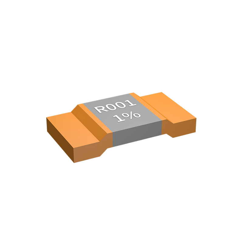
Thick film parts look settled on the datasheet, but if you track them over hundreds of hours at modest temperature swings, the resistance creeps in a way that isn't obvious from a single measurement. The glass matrix and the conductive particles expand and contract at slightly different rates, and the micro-welds between grains keep rearranging. That slow shuffle shows up as a soft upward or downward wander, often tens of parts per million, with occasional small jumps after thermal cycling.
Metal foil doesn't just start quieter; it tends to stay closer to where it began. The resistive element is a cold-worked alloy bonded to a ceramic substrate, so there aren't the same granular contacts fighting each other. The drift mechanism is more about stress relaxation in the first few hundred hours, and once that settles, the curve flattens noticeably. You still see tiny shifts from humidity or board flex, but they're usually an order of magnitude below what a typical thick film part produces under identical conditions.
The practical difference becomes clearer in precision dividers or reference scaling networks. A thick film resistor may test fine on arrival, yet six months later the ratio has moved enough to require a recalibration. With foil, the adjustment is less frequent, and the noise floor doesn't rise the same way with age. For circuits where long-term repeatability matters more than initial unit cost, that difference is what separates a stable reading from one that slowly drifts out of tolerance.
Kelvin Sensing Is Not Optional Below 10 Milliohms
When resistance values drop below 10 milliohms, even the shortest test leads introduce errors that swamp the measurement itself. A typical pair of meter probes can contribute 50 to 200 milliohms of lead resistance, which is an order of magnitude larger than the device under test. Two-wire readings in this range are essentially meaningless—you are measuring the leads, not the component. Kelvin sensing removes this problem by routing current through one set of contacts and sensing voltage through a separate pair, so the voltage drop across the target resistance is captured directly at its terminals.
The need for a four-terminal connection becomes non-negotiable because contact resistance at the probe tips also fluctuates with pressure, oxidation, and temperature. At 5 milliohms, a 10-milliohm variation in contact resistance produces a 200% error. Kelvin clips or dedicated four-wire fixtures force the current and voltage paths to meet only at the surface of the resistor under test, bypassing both the lead wire resistance and the contact interface. Trying to compensate for these effects in software is not practical below 10 milliohms—the thermal EMFs and noise alone can exceed the signal you are trying to resolve.
For anyone working with current-sense resistors, battery internal resistance, or PCB trace impedance, switching to Kelvin sensing is not a refinement but a prerequisite. A two-wire milliohm meter might show a stable reading, yet that reading will be dominated by the fixture rather than the sample. The boundary around 10 milliohms is where the uncertainty from ordinary leads overtakes the resolution of most handheld DMMs. Below that threshold, if you are not using a four-wire setup, you are not measuring resistance—you are measuring the limitations of your cables.
Self-Heating Curves You Can Actually Use
Most published self-heating curves are polished to the point of hiding the very details that matter in practice. The ones you can actually use often have a slight baseline drift, a sample mass that was rounded off, or an oven door opened two minutes early. That is not a flaw—it is reality. Overlay three or four of these imperfect runs and the true onset temperature becomes visible, not as a single circled number but as a band where heat generation starts to overtake heat losses.
A curve earns its place on your clipboard when it shows the sample center temperature, ambient temperature, and setpoint on the same time axis. The lag between setpoint and center is not just an artifact; it tells you how much thermal inertia your packaging or pile size is adding. When the center line keeps climbing after the external heating stops, that trailing rise is the first honest sign of self-heating. If you ignore that and wait for a flat line, you have already missed the useful warning.
Instead of chasing a perfectly smooth baseline, collect curves under two or three fill volumes or moisture levels. The spread between them gives you a practical safety margin, something no single average curve can provide. Set your alarm not at the average onset but at the lower edge of that spread. That way the curve is not just data—it becomes a decision tool you can rely on when the next batch is slightly different from the one in the report.
Solder Joint Stress and the Microvolt Price
A bent PCB or a slightly mismatched thermal expansion can push a solder joint into a state of residual stress that barely registers on a strain gauge, yet it silently adds a few microvolts to the signal path. In a 24-bit acquisition system where one LSB might be only 0.6 µV, that is not background noise—it is a systematic error hiding in plain sight.
The mechanism is rarely a single clean effect. Stressed solder alters the Seebeck coefficient at the copper-solder-lead junction, so any thermal gradient across the board turns the joint into a tiny thermocouple. At the same time, micro-cracks or grain boundary slip change local resistance, and the resulting current flow through imperfect contacts produces a small ohmic drop that drifts with time. Engineers often chase the wrong culprit, swapping amplifiers or adding filtering, while the real offset lives in the mechanical interface.
Paying the microvolt price means either designing the stress out—through flex reliefs, matched CTE materials, and controlled reflow profiles—or accepting it and calibrating after assembly. The latter is cheaper only if the stress remains stable; under thermal cycling or vibration it usually does not. For precision instruments, the cost of ignoring solder joint stress is measured not in dollars but in lost resolution and unexplained drift.
Matching the Shunt to Your Front-End Noise Floor
When selecting a shunt resistor for current measurement, the front-end noise floor sets the ultimate limit on how small a signal you can resolve. A shunt that's too large generates excessive voltage drop and heat, while one that's too small buries the signal under amplifier noise. The trick is to size the shunt so its Johnson noise and the amplifier's input-referred noise are roughly in the same ballpark. If the amplifier noise dominates, you're wasting dynamic range; if the shunt's thermal noise dominates, you're adding unnecessary power loss.
Start by looking at the amplifier's input-referred voltage noise density and the current you need to measure at the low end. The shunt's resistance should produce a voltage drop at that minimum current that sits above the amplifier's noise floor by a comfortable margin, but not so far above that you cook the resistor or ruin efficiency. For many precision front-ends, this lands the shunt in the milliohm range, where even tiny changes in layout and Kelvin connection matter more than the nominal resistance value.
Don't forget that the shunt's own thermal noise is proportional to the square root of resistance and temperature. Matching the shunt to your front-end noise floor isn't about hitting an exact number; it's about finding the resistance where the system noise is limited by the front-end, not by the shunt. That balance point gives you the best signal-to-noise ratio for the least amount of heat and voltage burden.
FAQ
It comes down to how well the resistor holds its value under changing temperature and load. High precision shunts use alloys like manganin or zeranin that exhibit very low temperature coefficients and minimal thermal EMF against copper. They also tend to be designed for four-wire measurement, so the voltage drop is sensed right at the resistive element rather than through the current-carrying leads.
Self-heating raises the element temperature, which shifts the resistance according to the TCR and can introduce drift that looks like a change in measured current. Derating the power by at least 50 percent, using larger packages with better heat spreading, and placing the shunt in a low-thermal-resistance path all help. If the shunt has a strong copper thermal connection to the board, the heat can be pulled away more effectively.
With two-terminal sensing, the voltage drop across the lead and solder joint resistance gets mixed into the measurement, and in low-value shunts that error can easily exceed the intended signal. Kelvin connections separate the current path from the sense path, so the sensing traces carry almost no current and read only the voltage developed across the resistive element itself.
Start from the maximum current you need to measure and the smallest voltage you can resolve reliably. A good target is to develop between 50 mV and 100 mV at full-scale current, balancing signal-to-noise ratio against power dissipation. For example, a 10 A shunt at 100 mV full scale would be 10 mOhm, and that dissipates 1 W at full load, which is manageable with proper derating.
Manganin, zeranin, and some nickel-chromium alloys are common because they have very low temperature coefficients and generate little thermal voltage against copper. Manganin is a classic choice for metrology-grade shunts due to its stability over time and predictable TCR curve. Thick film and metal strip are less stable, so they rarely appear in truly high precision applications.
Yes, layout can dominate the error budget. Sense traces should be routed as a differential pair, kept away from high-current paths, and connected exactly at the shunt's Kelvin terminals. Any ground plane cut or asymmetry between the sense lines can couple magnetic fields and create a false voltage. Thermal gradients across the board can also generate thermocouple effects if different metals meet at the sense points.
For metrology or critical industrial use, an annual verification against a known current source and a higher-accuracy reference shunt is typical. Lab environments with stable temperatures may extend that interval, while field equipment exposed to thermal cycling or humidity should be checked more frequently. The key is to monitor drift over time rather than trusting a one-time factory calibration.
Thermal EMF is a small voltage generated at the junction of two different metals when a temperature difference exists. In a shunt, the junction between the resistive alloy and the copper leads can generate microvolts to millivolts of error, which directly adds to the sensed voltage. Choosing materials that are thermoelectrically compatible with copper and keeping the two sense terminals at the same temperature minimizes this error.
Conclusion
Precision current sensing starts with more than a tight tolerance spec. A 0.1% resistor can still produce misleading readings if thermal drift, self-heating, or solder joint stress quietly shifts its value. Thick film parts tend to wander a few hundred ppm as temperatures cycle, while metal foil and wirewound alternatives hold much tighter, often under 30 ppm, making them better suited for repeatable measurements. Below 10 milliohms, four-wire Kelvin connections are non-negotiable; without them, lead and trace resistance easily overwhelms the shunt's own tiny resistance. Self-heating curves from the datasheet reveal how much power the part can dissipate before its resistance climbs, and that temperature rise directly becomes an error term in microvolts.
A practical selection flow looks at the front-end noise floor before settling on a resistance value. A larger shunt produces more signal but more heat and voltage drop; a smaller one keeps losses low but can bury the measurement in amplifier noise. Solder joint stress acts as a silent offset generator—uneven pad layouts or board flex can create thermocouple junctions at the terminations, costing several microvolts. Match the shunt's thermal EMF behavior and low ohmic value to the ADC's input range and noise density, then verify the board layout with Kelvin pads close to the element. The best high precision shunt is not simply the one with the lowest tolerance; it is the one whose drift, self-heating, stress sensitivity, and noise contribution align with the actual measurement range and environment.
Contact Us
Contact Person: Yuying Gao
Email: [email protected]
Tel/WhatsApp: +86 18926013721
Website: https://en.milliohm.net/